Risk is not a number!

Written By: Toby Nangle Global Co-Head of Multi Asset & Head of Asset Allocation, EMEA Columbia Threadneedle Investments

& Moira Gorman Client Director, LGPS Columbia Threadneedle Investments

Toby Nangle and Moira Gorman of Columbia Threadneedle Investments warn of the danger of over-reliance on statistical models when calculating risk

• “Risk” is a loaded word meaning different things to different people.
• No statistical model can predict consistently the future, but a portfolio risk framework can be used to be mindful of the lessons of the past.
• Being aware of the model risks in your risk framework is an essential prerequisite to discussing risk outputs. Risk on its own is not a useful statistic, it’s what you do with it that counts.

One of the problems when talking about “risk” is that it means very different things to different people. Risk is a multi-faceted notion, capturing a plethora of operational, political, economic and financial variables, all relating to the possibility of loss or reduction in purchasing power in an investment context. We have a large number of processes and checks to attempt to capture an estimation of these risks, and where possible seek to reduce or eliminate them for our clients. But in investment professional speak “portfolio risk” generally refers to a tiny subset of this broad definition of risk, otherwise known as “return volatility”.1

A portfolio that exhibits a lot of return volatility (perhaps one invested entirely in risky assets like equities) is understood as having a high level of investment risk, while a portfolio investment that exhibits very little return volatility (perhaps one invested entirely in less risky assets like short-dated government bonds) is, under this definition of risk, understood as having a low level of investment risk. This is very backwards-looking, and while it is unhelpful to say so, the thing about measures of return volatility is that they are quite volatile. Looking at the return volatility of the global equity market over the past 45 years makes the point well (Figure 1).

Figure 1: Annualised volatility of monthly price returns for the MSCI World Index 1970-2015 using 3.5-year rolling data windows of equally-weighted data

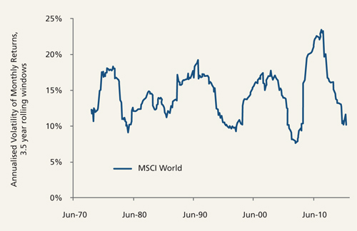
Source: Columbia Threadneedle Investments, December 2015

Return volatility tends to rise when prices fall and tends to fall when prices rise, although this is not exactly a linear process: Figure 2 plots the relationship between experienced annualised volatility of returns (aka risk) and annualised price returns since 1970. Targeting a specific level of experienced volatility by selling after reported historical volatility has risen, and buying after reported historical volatility has fallen, has hitherto proven a means of buying high and selling low.

Figure 2: Annualised returns vs annualised volatility of MSCI World Index 1970-2015 using 3.5-year rolling data windows

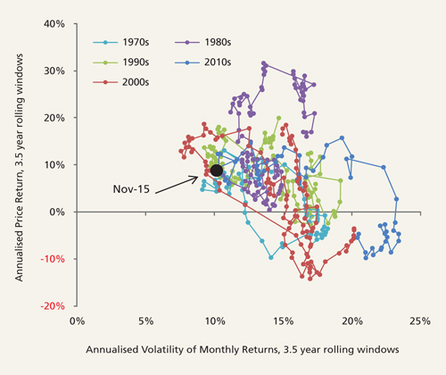
Source: Columbia Threadneedle Investments, December 2015

When investing we are less interested in what happened in the past than we are as to what will happen in the future. But no statistical model can predict the future consistently; model outputs should only be used to help us understand the lessons of the past. And so as a portfolio manager I regard our statistical risk models much as I would a wizened colleague with a perfect memory of the past who can perform complex calculations in their head, remembering not only the variance of asset returns, but also the correlation of the price returns of all of the potential individual assets that we might consider selecting for inclusion in a portfolio. This can be quite useful when we seek to interrogate a portfolio to see how it would have performed under different historical environments.

But while portfolio construction can be described in a highly quantitative manner, it is essentially forward-looking and qualitative. We use a variety of statistical engines to help us understand the return volatility that a portfolio would have enjoyed or suffered over different historical periods with historical asset volatility and correlation characteristics, but we can’t do more than qualitatively estimate the future environment. The process of interactions between risk models and a portfolio manager is much more important than the final number that any risk model spits out.

Risk models can use different data windows (most commonly, trailing 180 weeks, 60 months, or 120 months up to the present day), and can either equally-weight or exponentially-weight the volatility and correlation characteristics exhibited by portfolio assets to produce portfolio risk numbers. And different time-windows, periodicities and weighting methodologies will deliver different portfolio risk numbers for the same portfolio – all of which will be internally coherent. Furthermore, even for a model that looks at 180 weeks of data equally-weighted, there can still be big differences in the risk number depending on which day of the week a model takes its weekly data readings. Figure 3 shows that the annualised volatility calculated for global equities using Monday-to-Monday observations comes to 13.3% – a full two-and-a-half percentage points higher than the 10.8% annualised volatility calculated for global equities using Thursday-to-Thursday observations. Put another way, the overall risk number output of a Thursday-to-Thursday 180 week equally-weighted risk model for a leveraged portfolio with 125% exposure to equities would be the same as the overall risk number output of a Monday-to-Monday 180 week equally-weighted risk model for an unleveraged portfolio with 100% exposure to equities. Put simply, risk numbers quickly lose their relevance outside their very specific context.

Figure 3: Annualised volatility of weekly price returns for MSCI World Index for 180 weeks to November 2015 using different days of the week

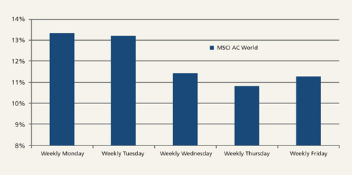
Source: Columbia Threadneedle Investments, December 2015

To help us understand the biases displayed by the choices we make in specifying the periodicity and data window, we track dashboards such as one in Figure 4 that show how correlations and volatility measurements change depending on tweaks to these inputs. Furthermore, we examine model estimates of portfolio risks using a variety of different data windows and periodicities as a test against our firm’s standard risk model. But most importantly, we never lose sight of the fact we cannot draw from past data a perfect model of future portfolio risks.

Figure 4: Comparing different levels of volatility and correlation outputs for given data periodicity and window size across selected high level asset classes

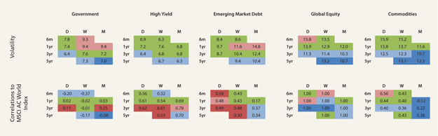
Source: Columbia Threadneedle Investments, December 2015

So when someone says that a portfolio has a volatility of 6% per annum, the appropriate response is not “that sounds high/low/about right”. The correct response is “What does that even mean, and how are you using that information in your portfolio?”

1. Return volatility here can be understood as a single standard deviation of the historical monthly returns multiplied by the square-root of twelve to annualise this monthly series. And so if the future stream of monthly returns has a similar distribution to the past stream of monthly returns, an annualised standard deviation of monthly returns equal to 6% per annum would indicate that one could have from a statistical point of view some confidence that the future return would be between +6% and -6% for two out of every three years, with the remaining year experiencing a return greater than +6% or less than -6%.