Tail risk in alternative risk premia

Written By: Moira Gorman Client Director Columbia Threadneedle Investments

& Benjamin Simonds Portfolio Manager Columbia Threadneedle Investments

Moira Gorman and Benjamin Simonds of Columbia Threadneedle Investments discuss the VaR characteristics associated with the different types of alternative risk premia, in particular the use of VaR in the management of a liquid alternatives portfolio

Managing tail risk has been an important part of modern portfolio construction for many years. Portfolio managers in the 1990s were introduced to the idea of “Value at Risk” (VaR), which measures the potential loss on an investment over a set time period given normal market conditions.

While the focus of VaR is on downside risk and potential loss, it is intended to address normal market risk vs any/all investment risk. At its introduction, VaR was a compelling but ultimately voluntary part of the risk management toolkit. Fast forward to 2016, and the idea of VaR has become so widespread that it is codified in UCITS regulations as the risk measure of choice, and one that should be an integral part of a manager’s portfolio construction process.

The goal of this article is to review the VaR characteristics associated with different types of alternative risk premia (also called alternative beta) products, focusing on the application of VaR in the management of a liquid alternatives portfolio.

There are three key elements in the calculation of VaR:

• Specified level of loss
• Fixed time period
• Confidence interval

VaR can be calculated for an individual asset or a portfolio of assets. Two major types of VaR calculations are: 1) analytical value at risk (AVaR) as well as 2) historical value at risk (HVaR).

AVaR calculates a portfolio’s mean and standard deviation, assumes a normal distribution, and then suggests what a negative event will be in light of those assumptions. AVaR requires no data beyond a volatility estimate.

HVaR, in contrast, makes no assumptions about the normality or lack thereof of a given return series and calculates the actual historical outcomes.

To give an example of both AVaR and HVAR: the S&P 500 Index over the last 10 years (as of the writing of this article) had an average daily return of 2.8 basis points and a daily standard deviation of 1.29%.

AVaR Calculation
To calculate a 99% AVaR, which is a 2.33 standard deviation event in the normal distribution, we would calculate 0.028% – 2.33 x 1.29% = -2.98%, or roughly -3%.

HVaR Calculation
For calculating HVaR, we would look at the actual observed daily returns of the S&P 500 over the past 10 years, and find that the 99th percentile event is
-3.89%, or roughly -4%.

In contrast to AVaR, HVAR may be most useful to investors seeking to understand the risks of a portfolio which is more likely to have left (or right) tail events more often than you would assume with normal distribution, as seen in Figure 1.

What do the differences in calculation mean for investors? The S&P 500’s fat-tailed nature, often documented, is more likely to produce a downside outlier event than we see demonstrated in a statistical “normal” distribution.

Figure 1: AVaR may not adequately capture left tail events (full curve and left tail detail)

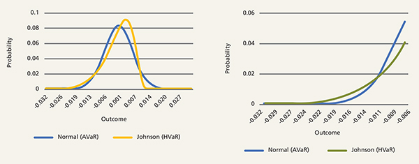
Source: Columbia Threadneedle Investments. Based on a theoretical series of returns with a 10% annualized return and 10% annualized volatility

Practitioners investing in alternative risk premia typically take a risk allocation approach (e.g., risk parity) rather than a capital allocation approach. Individual risk premia structures tend to exhibit significant volatility variability and idiosyncratic risk between one another so allocating based on these risk differences as opposed to simply adjusting the capital exposure is essential for creating a properly balanced portfolio. The varied use of leverage across different counterparties means one cannot look at a simple return or risk number when considering the risk of a prospective investment. Instead, investors in alternative risk premia should look at a scalable ratio, e.g. Sharpe ratio, rather than raw performance returns. To that point, in thinking about VaR, an investor also needs a scalable way to consider the relative tail risk of different strategies. We can use the HVaR and AVaR measures, and take the ratio of the two, to get a sense for how much of the risk in a given return series is focused in the left tail (downside). Any ratio greater than 1.0 would suggest that a given investment has more negative tail risk than a normal distribution, and any ratio less than one 1.0 suggests a given investment has less negative tail risk than a normal distribution.

In our view, the use of an HVaR/AVaR ratio is more powerful than relying on either of the underlying calculations singly because it is indifferent to the volatility of the series.

Moving on to alternative betas, we consider a sample of 211 different alternative beta indices listed in Bloomberg that fall into the categories of Equity, FX, Credit, Rates, Commodity, and Short Volatility. Grouping them by category, we observe in Figure 2 distributions of the HVaR/AVaR ratio.

Figure 2: Sample of 211 different alternative beta indicies listed in Bloomberg

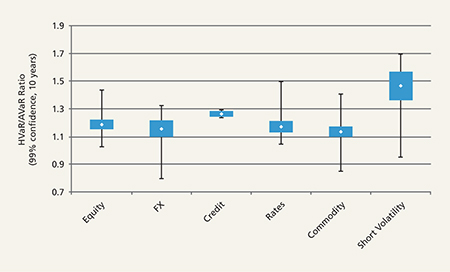
Source: Columbia Threadneedle and Bloomberg as of August 25, 2016. Calculations are based on 10-year average return and volatility data. HVaR is based on 10 years of returns

Several notes and observations may be made from Figure 2:

• The highest ratios (i.e. more left tail risk) by far fall into the Short Volatility category.
• The small range of Credit is due to the relatively small selection of series. We chose to separate Credit and Rates in order to preserve the observation that Credit series tend to have a relatively high ratio (i.e. more left tail risk).
• The remaining areas (Equity, FX, Rates and Commodities) all appear to have relatively low ratios (i.e. less left tail risk) with a wide range of possible outcomes.
• All of these, across alternative betas – with the exception of the short volatility strategies – compare very favourably with the traditional asset ratios. For example, the S&P HVaR/AVaR ratio of 1.31 (calculated over 10 years of daily data to 25 August 2016 at 99% confidence) is higher than the typical ranges for all except the short volatility group.

We extend this analysis out across various factor sub-categories, as displayed in Figure 3.

We note that:

• Momentum strategies tend to have higher downside potential than other equity strategies.
• Among currency strategies, FX Value stands out on the lower end.
• Commodity Carry appears on the lower end of the commodity strategies.

Figure 3: Distributions of HVaR/AVaR across a variety of factor sub-categories

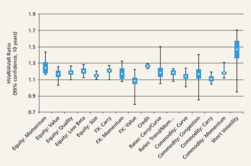
Source: Columbia Threadneedle and Bloomberg as of August 25, 2016. Calculations are based on 10-year average return and volatility data

What does this mean?
For a portfolio manager of alternative risk premia, these types of analyses can be a useful tool in portfolio construction. For example, a manager may decide to set a cap on the weighting to a specific risk premia style like short volatility strategies in their portfolio, or introduce a portfolio construction guideline that seeks to establish a set ratio of asset class weights based on the VaR of the constituent asset classes.

Similarly, a manager may look at the ratios of individual holdings within a given asset class and make similar adjustments. These types of guidelines may seek to offset exposures to assets with high fat-tail risk with assets with lower fat-tail risk, or seek a balanced distribution of ratios.

HVaR and AVaR both have limitations and practitioners are well-advised to consider these values in conjunction with stress testing and scenario analysis as a means of exploring portfolio tail risks. In conclusion, HVaR is a particularly relevant metric to manage more left tail prone investments like risk premia strategies. It is one of many tools available to practitioner’s in this space to help create the risk/return profile desired. Our DARP portfolio relies heavily on HVaR to maintain the overall portfolio risk target of 7.5% and to keep the individual exposures in line with our objectives.